This post describes the workings of Latent Semantic Analysis and the surrounding tools to get to an analysis.

Bag of words (BOW)

The bag of words model is one of the simplest representations of document content in NLP. The model consists of content split up into smaller fractions. For simplicity, we will be restricted to plain text. The model stores all present words in an unordered list. This means that the original syntax of the document will be lost, but instead we will gain flexibility in working with each word in the list. As an example, the operation of removing certain words or simply changing them would become much easier, since ordinary list operations can be used.

The BOW representation can be optimized even further if all words are translated to integers. This can be done by using a dictionary to store the actual words.

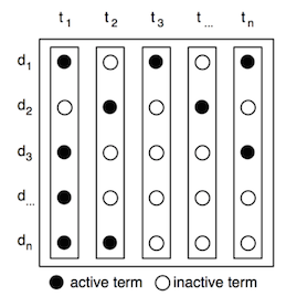
Document-term matrix

The document-term matrix is a basic representation of our group of documents (corpus) that consists of rows of words and columns of documents. Each matrix value consists of the weight for a specific term in a specific document. The calculation of the words can vary, but in this text, it will represent the number of times a word is present in the document. The advantage of having the corpus represented as a matrix is that we can perform computational calculations on it using linear algebra.

Latent Semantic Analysis

LSA is a vector-based method that assumes that words that share the same meaning also occur in the same texts (Landauer and Dumais, 1997:215). This is done by first simplifying the document-term matrix using Singular Value Decomposition (SVD), before finding close related terms and documents. This is done by using the principals of vector-based cosine similarities.

By plotting a number of documents and a query as vectors, it is possible to find the Euclidian distance between each document vector and a query vector. This can also be thought of as grouping together terms that relate to one another. This operation should, however, not be confused with clustering of terms, since each term in our case can be part of several groups.

In the following text, I will introduce the most important building blocks of LSA before piecing it all together in the end and show how to perform queues and extend a trained index.

The corpora as vectors

When our corpus is in the form of a document-term matrix, it’s simple to treat it as a vector space model, where we perceive each matrix column as a vector of word weights.

Since only a minor part of the words are used to represent each document, this means that the vectors mostly consist of zeroes, also called sparse vectors.

The advantage of representing each document as a vector is that we then have the ability to use geometric methods to calculate the properties of each document. When plotting the vectors in an n dimensional space, the documents that share the same terms tend to lie very close to each other. To demonstrate this, we will display a couple of vectors from a very minimalistic document- term matrix. This is because we are only able to visualize up to three dimensions in a three- dimensional world. Since paper only has two dimensions, we will simplify even further by only using two dimensions.

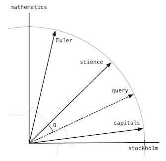
In the following the document vectors will be plotted. This means that the terms are equal to the dimensions used. Since we only have two dimensions, our term document matrix can only have two terms. We have randomly picked the terms “mathematics” and “Stockholm”. This will be our two dimensions. If we then have three documents that we want to plot, we will take the weight of the two terms in each of the three documents and plot them as vectors (from the center). If the first document is about Leonhard Euler, the next is about Scandinavian capitals, and the third is about science in Sweden, then plotting the three documents by the two terms would perhaps look like this:

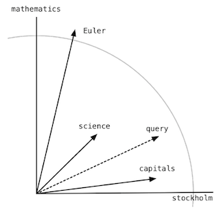
The length of the vectors tells us something about how many times the terms are present in each document. Let us say that the grey line marks a scale of 10, then the document about Euler would contain around 11-12 words about mathematics and around three words about Stockholm. The same principle goes into creating the rest of the vectors. In this way, we can plot any query onto the plane and see how close it is to any of our existing documents. This means that the closer two document vectors are, the closer their content is to each other. This again means that we want the angle to be as small as possible, and therefore we want cosine to be as big as possible. Since we are working with vectors, we know that we can calculate the angle between two vectors by

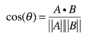
where A and B are the two vectors. This is referred to as the cosine similarity of the two vectors. To make this even simpler, we can normalize the vectors so that their length is always equal to 1. This means that we can reduce the above formula to

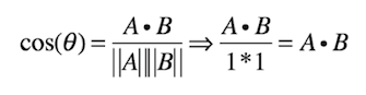
which is very easy to calculate on a large set of vectors. The method above is very important for finding similarities in large corpora. The result of the normalized vectors will render the model as follows:

The range of the cosine similarity is −1 to 1, where 1 indicates that the two vectors are exactly the same, 0 that the two vectors are independent and −1 that the two vectors are exactly opposite.

tf-idf

When using the values from the document-term matrix, commonly used words tend to have an advantage, because they are present in almost every document. To compensate for this, tf-idf (Term Frequency - Inverse Document Frequency) is very often used. The point of using tf-idf is to demote any often used words, like “some”, “and” and “i”, while promoting less used words, like “automobile”, “baseball” and “london”. This approach easily removes any commonly used words while promoting domain-specific words that are significant for the meaning of the document. By doing this, we can avoid using lists of stop- words to remove commonly used words from our corpus.

The model is comprised of two different elements. First, the Term Frequency (TF) part that is the number of times a term is represented in a document, while Inverse Document Frequency (IDF) is the number of documents in the corpus divided by the document frequency of a word, but inverted.

Because tf-idf uses the logarithmic scale for its calculations of IDF, the result cannot be negative. This means that the cosine similarity cannot be negative either. The range of a tf- idf cosine similarity is therefore 0 to 1, where 0 is not similar and 1 is exactly the same.

Singular Value Decomposition (SVD)

Finding document similarities by using vector spaces on a document-term matrix can often become a costly process. Since even a modest corpus is likely to consist of tens of thousands of rows and columns, a query on the model can prove to take up a lot of time and processing power. This is because each document vector has a length of all the terms in the matrix. Finding the closest vectors in all dimensions is not a small task. What singular value decomposition (SVD) gives us is the ability to perform two important tasks on our document-term matrix, namely reducing the dimensions of our matrix and in this process finding new relationships between the terms across our corpora. This will create a new matrix that approximates the original matrix, but with a lower rank (column rank).

The basic operation behind SVD is to unpack our matrix, promote non-linear terms and use this to reduce the size of our matrix without losing much quality. Then afterwards, the data is packed up again into a smaller, more efficient version. All of this while keeping the essence of our original matrix. A fortunate side-effect of this process is a tendency to bring the co- occurring terms closer together.

In the following sub-chapter, we will try to go a little deeper into the workings of SVD. If we have the M × N document-term matrix C, then we can decompose it into three components by the following

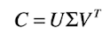
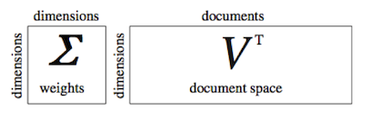
where U is an M × M matrix where the columns are the orthogonal eigenvectors of CC^T, V is an N × N matrix where the columns are the orthogonal eigenvectors of C^TC and Σ is an M × N zero matrix with the eigenvalues of CC^T (or C^TC) placed on the diagonal in descending order and then squared (Manning et al. 2008:408). These are known as the singular values of C

To reduce the size of our matrix without losing much quality, we can perform a low-rank approximation on matrix C. This is done by keeping the top k values of Σ and setting the rest to zero, where k is the new rank. Since Σ contains eigenvalues in descending order, and the effect of small eigenvalues on matrix products is small (Manning et al. 2008:411), the zeroing of the lowest values will leave the reduced matrix C' approximate to C. How to retrieve the most optimal k is not an easy task, since we want k top large enough to include as much variety as possible from our original matrix C, but small enough to exclude sampling errors and redundancy. To do this in a formal way, the Frobenius norm can be applied to measure the discrepancy between C and C_k (ibid.:410). A less extensive way is just to try out a couple of different k-values and see what generates the best results.

When reducing the rank of a document-term matrix, the resulting matrix C' becomes far more dense compared to the original matrix C, which means that although the dimensions of our original matrix C become smaller, the content of C' becomes more compact, thus requiring more computational power. Because of this, we do not reduce the dimensions of C.

Piecing it together

Once we have applied tf-idf and SVD to our document-term matrix, we can again apply the cosine similarity procedures. With the rank reduction of the original matrix, what we have is an approximation of the document-term matrix, with a new representation of each document in our corpus. The idea behind LSA is that the original corpus consists of a multitude of terms that in essence have the same meaning. The original matrix can in this sense be viewed as an obscured version of the underlying latent structure we discover when the redundant dimensions are forced together.

Another important advantage of LSA is its focus on trying to solve the synonymy and polysemy problem. Synonymy describes the instance where two words share the same meaning. This could be “car” and “automobile”, “buy” and “purchase”, etc. This can cause problems when searching for documents with certain content, only to receive results not bearing the synonyms of the query text. As for polysemy, this describes words that have different meanings depending on the context. This could be “man” (as in human species or human males or adult human males), “present” (as in right now, a gift, to show/display something or to physically be somewhere (Wikipedia, 2012)), etc. In cases of polysemy, documents that have nothing to do with the intent of the query can easily become falsely included in the result.

When looking at the vector space model, the problem of synonymy is caused by the query vector not being close enough to any of the document vectors that share the relevant content. Because of this, the user that makes the query needs to be very accurate in searching, or the search engine needs to have some kind of thesaurus implemented. The latter can be a very costly and inaccurate affair. When putting our original document-term matrix through LSA, synonyms are usually not needed, since similar terms should be grouped together by the lowering of rank. Since applying LSA also lowers the amount of “noise” in the corpus, the amount of rare and less used terms, should also be filtered out. This of course only works if the average meaning of the term is close to the real meaning. Otherwise, since the weight of the term vector is only an average of the various meanings of the term, this simplification could introduce more noise into the model.

Performing searches

To perform queries on a model, the query text must be represented as a vector in the same fashion as any other document in the model. After the query text has been converted to a vector representation, it can be mapped into the LSA space by

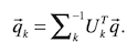
where q^(arrow) is the query vector and k is the number of dimensions. To produce the similarities between a query and a document or two documents or between two words, we can again use cosine similarities.

Since a query can be represented as just another document vector, the equation above also works for adding new documents to the model. This way we do not have to rebuild the entire model every time a new document needs to be indexed. This procedure is referred to as “folding-in” (Manning et al. 2008:414). Of course with folding-in, we fail to include any co- occurrences of the added document. New terms that are not already present in the model will be ignored. To truly include all documents in the model, we have to periodically rebuild the model from scratch. This is, however, usually not a problem since a delta-index can easily be rendered in the background and be switched in when ready.

Comparing two terms

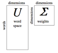
We also know previously that the matrix U (the word space) consists of tokens and the number of dimensions of the SVD, while matrix Σ (the weights) is an m × m matrix where m is also the number of dimensions of the SVD.

To compare two terms, we know from Deerwester that the dot product between the i^(th) column and the j^(th) row of matrix UΣ will give us the similarity between the two words chosen. This is because the UΣ matrix consists of the terms and the weights of those terms in the SVD.

Comparing Two Documents

The approach of comparing two documents is similar to comparing two terms. The difference is that instead of using matrix UΣ, we instead take the dot product between the i^(th) and j^(th) rows of the matrix VΣ and that gives us the similarity between the two documents.

Comparing a Term and a Document

The approach of comparing a term and a document is a little more different than in the method used above. It will simply come down to the weight of a specifc term on a specific document. For this we will need the values from both UΣ and VΣ, but since we are going to combine the result, the values of the 2 matrices will have to be divided by 2.

To complete the operation, the dot-product between the i^(th) and the j^(th) row of matrix UΣ^(1/2) and the j^(th) row of matrix VΣ^(1/2) (Deerwester, 1990:399)